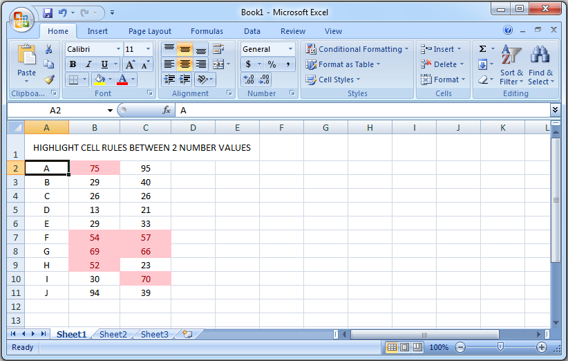
Conditional Formatting : Highlight Cell Rules Between 2 Numeric Values

Conditional Formatting : Highlight Cell Rules Between 2 Numeric Values.

Hi friends, on this occasion we will discuss how to mark a particular cell using Conditional Formatting. This method is useful for sorting numbers with a certain value limits specified. Let's say we have 20 different numbers, and we will highlight it on a limited number with a value between 40 and 80. Numbers within the range between 40 and 80 are numbers that we will highlight. This will be useful when we want the filtering of certain values ​​as a result of a sorted value.

Let's start by creating a cell range with 3 columns and 10 rows field. Let us assume that the first column as the identity of the owner of the value, while the second and third column is the value of two different sources. We will highlight the values ​​contained in column 2 and column 3 and filter them so that we get the number ranges between 40 and 80. Below is a spreadsheet that we will create.

Creating cell ranges.

1. Create a range between A1 to C11 as shown on the picture above. We will create a range that will carry about 10 lines as an example.
2. Highlight the range so the two columns that contains the numbers highlighted. After that, we going to Conditional Formatting with the sequence of steps : Conditional Formatting > Highlight Cells Rules > Between...
   
3. In the "Between" window, there are two text boxes with the name "Format cells that are BETWEEN:", fill in the ranges of numbers that we want. Suppose we want the ranges between 40 and 80. On the right of the dropdown menu, there is a cell format option. Just an example, we use the default option is "Light Red Fill with Dark Red Text" and then click OK. You can choose another format such as border and variations of text by selecting the "Custom Format".
   
4. As a result, the numbers which are in the ranges between 40 and 80 highlighted with the color we specified earlier. As shown in the picture below.
   

We can change the Conditional Formatting rules any time by clicking Conditional Formatting > Manage Rules. Hope this tutorial about How to Highlight Cell Rules Between 2 Numeric Values Using Conditional Formatting is helpful. Thanks Excelsor !